Efficient signal propagation

Modeling signal propagation efficiently is essential for scalable wireless simulation. When a simulated radio entity transmits a signal, the SWANS Field entity must deliver that signal to all radios that could be affected, after considering fading, gain, and pathloss. Some small subset of the radios on the field will be within reception range and a few more radios will be affected by the interference above some sensitivity threshold. The remaining majority of the radios will not be tangibly affected by the transmission.

ns2 and GloMoSim implement a naïve signal propagation algorithm, which uses a slow, $O(n)$, linear search through all the radios to determine the node set within the reception neighborhood of the transmitter. This clearly does not scale as the number of radios increases. ns2 has recently been improved with a grid-based algorithm [6]. We have implemented both of these in SWANS. In addition, we have a new, more efficient algorithm that uses hierarchical binning. The spatial partitioning imposed by each of these data structures is depicted in Figure 2.

Figure 2: Alternative spatial data structures for radio signal propagation: Efficient signal propagation is critical for wireless network simulation performance. Hierarchical binning of radios on the field allows location updates to be performed in expected amortized constant time and the set of receiving radios to be computed in time proportional to its size.

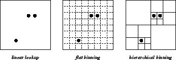In the grid-based or flat binning approach, the field is sub-divided into a grid of node bins. A node location update requires constant time, since the bins divide the field in a regular manner. The neighborhood search is then performed by scanning all bins within a given distance from the signal source. While this operation is also of constant time, given a sufficiently fine grid, the constant is sensitive to the chosen bin size: bin sizes that are too large will capture too many nodes and thus not serve their search-pruning purpose; bin sizes that are too small will require the scanning of many empty bins, especially at lower node densities. A reasonable bin size is one that captures a small number of nodes per bin. Thus, the bin size is a function of the local radio density and the signal propagation radius. However, these parameters may change in different parts of the field, from radio to radio, and even as a function of time, for example, as in the case of power-controlled transmissions.

We improve on the flat binning approach. Instead of a flat sub-division, the hierarchical binning implementation recursively divides the field along both the $x$ and $y$-axes. The node bins are the leaves of this balanced, spatial decomposition tree, which is of height equal to the number of divisions, or $log_4(\frac{field\ size}{bin\ size})$. The structure is similar to a quad-tree, except that the division points are not the nodes themselves, but rather fixed coordinates. Note that the height of the tree changes only logarithmically with changes in the bin or field size. Furthermore, since nodes move only a short distance between updates, the expected amortized height of the common parent of the two affected node bins is $O(1)$. This, of course, is under the assumption of a reasonable node mobility that keeps the nodes uniformly distributed. Thus, the amortized cost of updating a node location is constant, including the maintenance of inner node counts. When scanning for node neighbors, empty bins can be pruned as we descend spatially. Thus, the set of receiving radios can be computed in time proportional to the number of receiving radios. Since, at a minimum, we will need to simulate delivery of the signal at each simulated radio, the algorithm is asymptotically as efficient as scanning a cached result, as proposed in [2], even assuming perfect caching. But, the memory overhead of hierarchical binning is minimal. Asymptotically, it amounts to $\lim_{n\to\infty}\sum_{i=1}^{log_4 n}\frac{n}{4^i}=\frac{n}{3}$. The memory overhead for function caching is also $O(n)$, but with a much larger constant. Furthermore, unlike the cases of flat binning or function caching, the memory accesses for hierarchical binning are tree structured and thus exhibit better locality.